
This is the notes for Chapter 5.4, mainly about ship waves.
ship waves
At sufficiently large distance behind the ship the crest curvature is not large, and our slowly varying assumptions will apply.
We regard disturbance as fixed at the origin, with a uniform current \((U_1,0)\) flowing past. The Doppler relation is then \[ \begin{equation} \omega=U_1 k_1+\sigma=U_1 k_1+\sqrt{g k } \end{equation} \] in deep water, neglecting surface tension, with \(U_1\) now constant. Therefore, the stationary phase occurs at \(\omega=0\). It follows that, the rays equations are \[ \begin{equation} \frac{\mathrm{d} x_1}{\mathrm{~d} t}=U_1+\frac{1}{2} \sqrt{\left(\frac{g}{k}\right)}\frac{k_1}{k} ;\quad \frac{\mathrm{d} x_2}{\mathrm{~d} t}=\frac{1}{2}\sqrt{\left(\frac{g}{k}\right)} \frac{k_2}{k} \end{equation} \]
--- note ----------------------
Q: how to get rays equations?
A: the dispersion relation are \[ \omega=U_1 k_1+\sqrt{g k} \quad, k=\sqrt{k_1^2+k_2^2} \]
The group velocity is \[ \begin{aligned} \overrightarrow{c_g}=\nabla_k \omega & =\left(\frac{\partial}{\partial k_i} \vec{e}_{k_i}\right) \omega \\ & =U_1 \vec{e}_{k_1}+\frac{\partial}{\partial k_1}(\sqrt{g k}) \vec{e}_{k_1}+\frac{\partial}{\partial k_2}(\sqrt{g k}) \vec{e}_{k_2} \\ & =U_1 \vec{e}_{k_1}+\frac{1}{2} \sqrt{\frac{g}{k}} \frac{k_1}{k} \vec{e}_{k_1}+\frac{1}{2} \sqrt{\frac{g}{k}} \frac{k_2}{k} \vec{e}_{k_2} \end{aligned} \] therefore \[ \begin{aligned} & c_{g_1}=U_1+\frac{1}{2} \sqrt{\frac{g}{k}} \frac{k_1}{k} \\ & c_{g_2}=\frac{1}{2} \sqrt{\frac{g}{k}} \frac{k_2}{k} \end{aligned} \] The rays are \[ \left\{\begin{array}{l} \frac{d x_1}{d t}=c_{g_1} \\ \frac{d x_2}{d t}=c_{g_2} \end{array}\right. \]
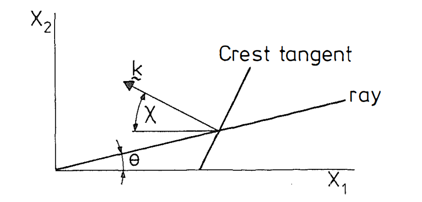
on the rays \[ \begin{equation} \frac{\mathrm{d} k_1}{\mathrm{~d} t}=0, \frac{\mathrm{~d} k_2}{\mathrm{~d} t}=0 \end{equation} \] in other words, \(k_1,k_2\) and hence \(k\) are constant on each ray and from \[ \begin{equation} \frac{\mathrm{d} x_2}{\mathrm{~d} x_1}=\text { constant }=\tan \theta \end{equation} \] we write \[ \begin{equation} \mathrm{k}=(-k \cos \chi, k \sin \chi) ; \end{equation} \] the angles \(\chi\) and \(\theta\) are shown in fig. 1, the minus in \(k_1\) allows for the fact that the waves must travel to the left to balance the flow \(U_1\) to the right.
Combining the (2) and (3) \[ \begin{equation} \tan \theta=\frac{\frac{1}{2}\sqrt{\frac{g}{k}}\sin \chi}{U_1-\frac{1}{2} \sqrt{\frac{g}{k}}\cos \chi} \end{equation} \] Back to \((1)\), stationary phase indicates \(\omega=0\), gives \[ \begin{equation} U_1 \cos \chi=\sqrt{\frac{g}{k}} \end{equation} \] therefore \[ \begin{equation} \tan \theta=\frac{\frac{1}{2} \sin \chi \cos \chi}{1-\frac{1}{2} \cos ^2 \chi} . \end{equation} \] Simplifying it \[ \begin{equation} \tan \theta=\frac{\frac{1}{2} \tan \chi}{\frac{1}{2}+\tan ^2 \chi} \end{equation} \] which is a quadratic for \(\chi\) when \(\theta\) is given \[ \begin{equation} \tan ^2 \chi(2 \tan \theta)-\tan \chi+\tan \theta=0 \end{equation} \] with roots \[ \begin{equation} \tan \chi=\frac{1 \pm \sqrt{1-8 \tan ^2 \theta}}{4 \tan \theta} . \end{equation} \]
relation between wave number \(N\) and length \(s\)
the distance \(d\;s\) is greater than \(\lambda\)
note that this is \(k-\text{plane}\)
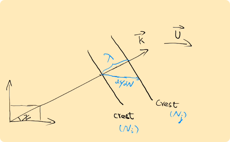
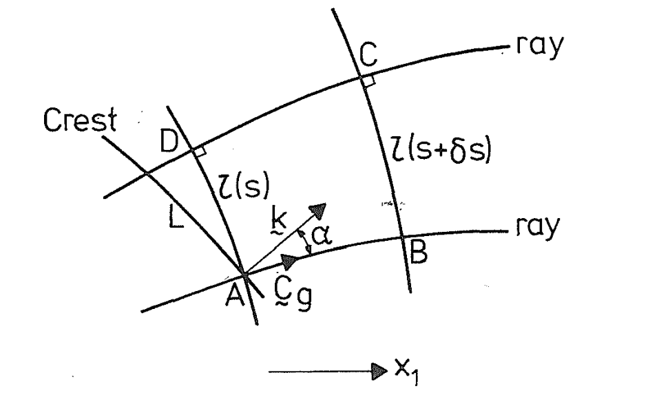
Counting wave crests along a ray, the relation between crests and rays is given by \[ \begin{equation} \frac{\mathrm{d} s}{\mathrm{~d} t}=\sqrt{\left(\frac{\mathrm{d} x_1}{\mathrm{~d} t}\right)^2+\left(\frac{\mathrm{d} x_2}{\mathrm{~d} t}\right)^2}=C_g \end{equation} \] The elementary number of waves \(d N\) in length \(ds\) is \(ds\) divided by the distance between two crests along the ray, as shown in above. Thus \[ \begin{equation} \mathrm{d} N=\frac{\mathrm{d} s}{(\lambda / \cos \chi)} \end{equation} \] where \(\chi\) is the angle between \(\bf{k}\) normal to the crests, and \(\mathbf{C}_g\) parallel to the ray, so that \[ \begin{equation} \begin{aligned} & \frac{\mathrm{d} N}{\mathrm{~d} s}=\frac{k}{2 \pi} \frac{\mathbf{k} \cdot \mathbf{C}_{\mathrm{g}}}{k C_{\mathrm{g}}}=\frac{\mathbf{k} \cdot \mathbf{C}_{\mathrm{g}}}{2 \pi C_{\mathrm{g}}}, \\ & \frac{\mathrm{~d} N}{\mathrm{~d} t}=\frac{\mathrm{d} N}{\mathrm{~d} s} \frac{\mathrm{~d} s}{\mathrm{~d} t}=\frac{\mathbf{k} \cdot \mathbf{C}_{\mathrm{g}}}{2 \pi} \end{aligned} \end{equation} \]
--- note ------------------------------------
\(\mathbf k\) is normal to crests, and \(\mathbf{C}_g\) parallel to rays.
note for (14) \[ \begin{aligned} & \lambda=\frac{k}{2 \pi} \\ & \cos \chi=\frac{\mathbf{k} \cdot \mathbf{C}_g}{k C_g} \end{aligned} \]
note that \(C_g=\frac{ds}{dt}\)
\(N\) is a scalar, represents the wave crest counter. Stated equivalently, \(N\) quantities the number of complete wave traversed along a ray. This may also be interpreted as the wave's "phase" expressed in units of cycles: \[ \begin{equation} N=\frac{\text{Total Phase}}{2\pi} \end{equation} \]
Let's now revisit \((11)\), the limiting value of \(\theta\) is such that the expression under the square root vanishes. We call it \(\theta_c\) \[ \begin{equation} \tan ^2 \theta_c=\frac{1}{8} ; \quad \theta_c=19^{\circ} 28^{\prime} \end{equation} \] For angles \(\abs{\theta}<\theta_c\) there are two roots of \(\chi\) for each \(\theta\), and there are no waves outside the wedge \(\abs{\theta}\leq\theta_c\). We use the expression for, \((14)\). For this we need \[ \begin{equation} \mathbf{k} \cdot \mathbf{C}_{g}=(-k \cos \chi, k \sin \chi) \cdot\left(U_1-\frac{1}{2} \sqrt{\frac{g}{k}}\cos \chi, \frac{1}{2} \sqrt{\frac{g}{k}} \sin \chi\right) \end{equation} \] Using \((7)\) \[ \begin{equation} \begin{aligned} \mathbf{k} \cdot \mathbf{C}_g & =\frac{g}{U_1 \cos ^2 \chi}\left(-\cos \chi+\frac{1}{2} \cos ^3 \chi+\frac{1}{2} \cos \chi \sin ^2 \chi\right) \\ & =-\frac{g}{2 U_1 \cos \chi} \end{aligned} \end{equation} \] We also need \[ \begin{equation} \begin{aligned} C_{\mathrm{g}} & =\sqrt{\left(U_1-\frac{1}{2}\sqrt{\frac{g}{k}} \cos \chi\right)^2+\left(\frac{1}{2}\sqrt{\frac{g}{k}} \sin \chi\right)^2} \\ & =U_1 \sqrt{1-\frac{3}{4} \cos ^2 \chi} . \end{aligned} \end{equation} \] Substituting into \(d N/d s\) and integrating \[ \begin{equation} N=\text { constant }-\frac{g s}{4 \pi U_1^2 \cos \chi \sqrt{1-\frac{3}{4} \cos ^2 \chi}} . \end{equation} \] A typical line of constant phase is shown below. The two systems of waves from the two roots for \(\chi\) are known as 'transverse' and 'diverging' and meet in the single root along the wedge line, which is another form caustic.
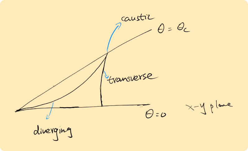
For real ship waves, there is actually a phase difference corresponding to a quarter of a wavelength along \(\theta=\theta_c\) between the two sets of waves, and the true pattern is shown below. This phase difference cannot be predicted by a theory of the type presented here, which depends on averaging and which pays no attention to the actual mechanics of the generation of the wave. It can be predicted by Fourier Transform methods, which are much more sophisticated mathematically.
wave action
The idea was originated from a technique known as Calculus of Variations, in the form which it is often used in Langrangian Mechanics. Here, we define wave action \(A\) by \[ \begin{equation} A=\frac{E}{\sigma}=\frac{2 T}{\sigma} \end{equation} \] in linear waves, where \(T\) is the kinetic energy. in non-linear systems, \(E\) is not equal to \(2T\). When there is a current we shall find that, neglecting friction effects, \(A\) is conserved even though \(E\) is not. Another form definition is \[ \begin{equation} A=\frac{I}{k}=\frac{I}{2 \pi} . \end{equation} \] where vector \(\mathbf{I}\) is \(2T/c=2Tk/\sigma=Ak\). The vector \(\mathbf{I}\) has been interpreted in two ways, as average mass flux or here, average wave momentum per unit surface area. The wave action equation is \[ \begin{equation} \frac{\partial A}{\partial t}+\operatorname{div}\left(\mathbf{C}_g A\right)=0 \end{equation} \]
--- note --------------------------------------------------------
wave crest and rays and wave number vector
The tangent to the rays aligns with the direction of the group velocity, wave vector \(\mathbf k\) is perpendicular to crest or wave front
We now refocus our attention on the amplitude considerations in ship waves. Our problem is steady, so \(\partial A/\partial t\) vanishes, and \(\mathbf{C}_g\) with components \(C_{gr}\), \(C_{g\theta}\) in the radial and transverse directions, therefore the wave action equation becomes \[ \begin{equation} \frac{1}{r} \frac{\partial}{\partial r}\left(A r C_{\mathrm{gr}}\right)+\frac{1}{r} \frac{\partial}{\partial \theta}\left(A C_{\mathrm{g} \theta}\right)=0 . \end{equation} \] The rays are radial lines. parallel to \(\mathbf{C}_g\), so \(\mathbf{C}_{g\theta}=0\) everywhere, and \((24)\) integrates: \[ \begin{equation} A r C_{\mathrm{gr}}=A r C_{\mathrm{g}}=\mathrm{constant} \end{equation} \] On any particular ray \(k\) and so \(C_g\) is constant and \[ \begin{equation} A \propto \frac{1}{r} \end{equation} \] or amplitude \[ \begin{equation} a \propto \frac{1}{r^{1 / 2}} \end{equation} \]
--- note ----------------------------------------------
Q: why \(a \propto \frac{1}{r^{1 / 2}}\)
A: \(a\) is the amplitude, we has the average kinetic energy \[ T=\frac{1}{4} \frac{\rho a^2 \sigma^2}{k \tanh k d}=\frac{1}{4} \rho g a^2 \] therefore \(a \propto \sqrt T\) , from \((21)\) \(A \propto T\) since \(\sigma\) is constant when \(k\) is fixed. Thus \[ a \propto \sqrt {T} \propto \sqrt{A} \propto \frac{1}{\sqrt r} \]
This formula is not correct close to the edge of the wedge where we have two interacting sets of waves, and in fact along \(\theta= \pm \theta_c\)
\[ \begin{equation} a \propto \frac{1}{r^{1 / 3}} \end{equation} \] but the Fourier Transform method is necessary to establish this result.
Real ship produce a wave pattern which roughly resembles that made by a positive disturbance of the type we have discussed at the bow, with a similar but negative disturbances at the stern. One possibility is that at a suitable speed, crests of the transverse waves made by the bow are at the same positions as the troughs of those made by the stern. The transverse waves are then largely cancelled and the resistance is reduced. This will happen if the effective length \(L\) of the ship is an integer multiple of the wavelength, \(L=N \;2\pi/k\). Along the ray \(\theta=0\) the two roots of \(\chi\) from \((11)\) are \(0\) and \(\frac{1}{2}\pi\), the former clearly corresponding to the transverse waves giving \[ \begin{equation} k=\frac{g}{U_1^2} \end{equation} \] from \((7)\). So cancellation occurs at \[ \begin{equation} \frac{U_1}{\sqrt{g L}}=\frac{1}{\sqrt{2 \pi N}} \end{equation} \] The non-dimensional number \(U_1/\sqrt{gL}\) is known as Froude Number.
In water of finite depth, the most noticeable feature is that as depth \(d\) reduces or as \(U_1\) increase, increasing the wavelength, the wedge angle increases until at \[ \begin{equation} F r=\frac{U_1}{\sqrt{g d }}=1 \end{equation} \] \(Fr\) is another form of Froude number, and (5.62) says that the ship speed \(U_1\) has reached the critical speed \(\sqrt{g d}\) which is the maximum possible speed of gravity waves, and where the group velocity \(c_{\mathrm{g}}=c\), the phase velocity. At lower speeds the wave energy is falling behind the ship. Viewed from the ship the wave crests have zero crest speed. Looking straight back, the transverse waves are travelling at speed \(U_1\) towards the ship and being swept back at speed \(U_1\) by the current. Their energy is travelling at speed \(c_{\mathrm{g}}<U_1\) towards the ship but is also being swept back at speed \(U_1\) by the current, and so, falls back, allowing a train of waves to form. As \(U_1\) reaches \(\sqrt{g d}\) so \(c_g\) reaches \(U_1\) and the transverse wave energy builds up near the ship giving an almost two-dimensional wave but not leaving anything downstream. This can be seen in Fig. 5.14. If \(U_1\) now increases further, transverse waves cannot keep up with the ship, since they would be beyond their fastest possible speed, and so there are no transverse waves. There is still a diverging wave pattern and as \(U_1\) continues to increase the wedge angle decreases again.
finite depth \(d\)
For the stationary phase \[ \begin{equation} \omega=0=U_1 k_1+k \sqrt{g d} \end{equation} \] then it follows that \[ \begin{equation} Fr \cos\chi =1 \end{equation} \] The rays equation give \[ \begin{equation} \begin{aligned} \frac{\mathrm{d} x_2}{\mathrm{~d} x_1}=\tan \theta &=\frac{\frac{k_2}{k} \sqrt{ gd}}{U_1+\frac{k_1}{k} \sqrt{ gd}} \\ & =\frac{\sin \chi}{F r-\cos \chi}\\ &=\frac{1}{\sqrt{F r^2-1}} \end{aligned} \end{equation} \] Thus for a given \(Fr\) there is only one value of \(\tan \theta\) and only one ray.